ETL & ELT

Column Operations & Graph Traversals

This article builds upon and refer to data from my previous article, describing a demonstrator from various data sources to a queryable knowledge graph.

Your pipeline loads customer data from four different sources. Orders from a CSV, products from Excel, tickets from a SQL endpoint, and customer master data from Parquet. Different column names, different conventions, different systems. You know the drill!

Silly, “mandatory”, illustration from my friend GPT. And because watercolours on the bus is a bit tricky.

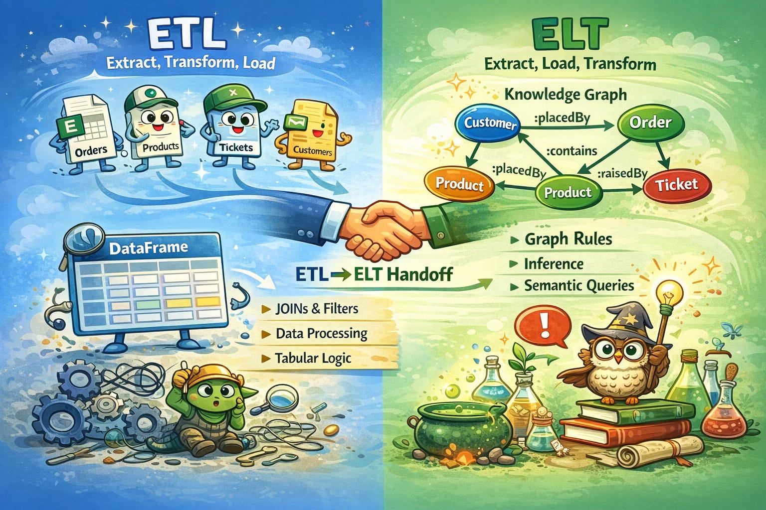
Now you need to derive some facts. Which customers purchased premium products? Which customers have orders, but no tickets? Which products should be classified as budget vs. premium based on their price?

If you’re a data engineer, you reach for Polars. Maybe dbt. You transform the data before it lands in the target system. That’s ETL (Extract, Transform, Load), it’s what you’ve been doing all the time, and it works well. Until the transformation you need is a multi-hop traversal across entities that live in different source systems.

That’s where graphs come in!

Extract, Transform, Load

Let’s make this concrete. Say you want to classify products as “Premium” (unit price > 500) or “Budget” (price <= 100). In Polars, this is straightforward:

import polars as pl

df_products = pl.read_excel("data/products.xlsx")

df_products = df_products.with_columns(
  pl.when(pl.col("price") > 500)
    .then(pl.lit("Premium"))
    .when(pl.col("price") <= 100)
    .then(pl.lit("Budget"))
    .otherwise(pl.lit("Standard"))
    .alias("tier")
)

Clean and familiar! You can see the logic, test it, and run it fast. The classification happens before the data enters the knowledge graph. For single-column, single-table operations like this, Polars is a great tool!

Where DataFrames hit the wall

Now try something slightly harder. Which customers purchased a premium product and raised a critical support ticket?

Think about what that requires:

1. Join orders to customers (orders.csv uses cust_ref, customers.parquet uses customer_id)

2. Join orders to products (orders.csv uses prod_code, products.xlsx uses sku)

3. Filter products where price > 500

4. Join customers to support tickets (support_tickets.csv uses client_id)

5. Filter tickets where severity = “critical”

6. Intersect the two result sets

# Step 1-3: customers who purchased premium products
df_premium_buyers = (
  df_orders
  .join(df_products, left_on="prod_code", right_on="sku")
  .filter(pl.col("price") > 500)
  .join(df_customers, left_on="cust_ref", right_on="customer_id")
  .select("customer_id", "full_name")
  .unique()
)

# Step 4-5: customers with critical tickets
df_critical_tickets = (
  df_tickets
  .filter(pl.col("severity") == "critical")
  .join(df_customers, left_on="client_id", right_on="customer_id")
  .select("customer_id", "full_name")
  .unique()
)

# Step 6: intersection
df_result = df_premium_buyers.join(df_critical_tickets, on="customer_id")

That’s six operations across four DataFrames, three different foreign key names, and you had to manage the harmonisation yourself. It works, but notice what happened: you’re essentially traversing a graph in tabular operations. Each JOIN is a hop, and as the hop increase, the complexity explodes.

Now add another requirement: only include customers whose premium product order was placed after their critical ticket was opened. Now you need temporal ordering across the intersection. The DataFrame chain gets longer, more fragile, harder to test.

This is the pattern where tabular transformations start to feel like the wrong abstraction. You’re fighting the data model, not working with it.

Extract, Load, Transform

Now, let’s have a look at the same problem by using graph transformations after load. The raw data has already been loaded, each source mapped into the same knowledge graph through OTTR templates, column names harmonised, IRIs constructed. The graph already knows that an order is :placedBy a customer and :contains a product. These things are not JOINs, they are edges!

Datalog

In the full demo at my repository data-engineering-to-knowledge-engineering, the transitive “purchased” relationship (the one that took two JOINs in Polars) is a single Datalog rule:

[?customer, :purchased, ?product] :-
  [?order, :placedBy, ?customer],
  [?order, :contains, ?product] .

And product classification is like this:

[?product, rdf:type, :PremiumProduct] :-
  [?product, rdf:type, :Product],
  [?product, :unitPrice, ?price],
  FILTER(?price > 500) .

When you call m.infer(rules), the reasoning engine materialise all the derived triples (adds new facts/statements to your graph). From that point on, :purchased and :PremiumProduct are just there. Queryable like any other fact in the graph!

Now, the hard question. Customers who bought premium products and raised critical tickets!

SELECT ?name
WHERE {
  ?customer :purchased ?product ;
    rdfs:label ?name .
  ?product a :PremiumProduct .
  ?ticket :raisedBy ?customer ;
    :priority "critical" .
}

No JOINs or foreign key juggling. The traversal across four entity types reads like a sentence. And adding the temporal constraint? One line:

FILTER(?order_date > ?ticket_date)

This is not just syntactic sugar. It’s fundamentally different approach to multi-hop transformations. In a DataFrame pipeline, you plan and execute each hop manually. In a graph, you describe the pattern you’re looking for and the engine traverses it for you.

SPARQL CONSTRUCT transformations

SPARQL¹ gives you another way to transform data inside the graph. A CONSTRUCT query creates new triples from existing ones:

PREFIX : <http://data.treehouse.example/>

CONSTRUCT {
  ?customer :purchasedPremium ?product .
}
WHERE {
  ?order :placedBy ?customer ;
    :contains ?product .
  ?product :unitPrice ?price .
  FILTER(?price > 500)
}

This produces a graph. The result is a set of triples you can merge back into the model using m.update(). The power is composability: you can chain CONSTRUCT queries, each one adds new facts, and the next query can use those facts. It’s transformations all the way down, and they all operate on the same unified graph.

In DataFrames, you would need to manage intermediate results, decide where to store them, and wire each step’s output to the next step’s input. In the graph, the intermediate results are the graph.

SHACL Rules

This is where it gets really interesting! SHACL Advanced Features (SHACL-AF) lets you define transformation rules as a part of your shapes. The same shapes you use for validation! A SHACL Rule is a CONSTRUCT query attached to a SHACL shape.

:PremiumProductRule
  a sh:NodeShape ;
  sh:targetClass :Product ;
  sh:rule [
    a sh:SPARQLRule ;
    sh:construct """
      CONSTRUCT {
        $this a :PremiumProduct .
      }
      WHERE {
        $this :unitPrice ?price .
        FILTER(?price > 500)
      }
    """ ;
  ] .

The $this variable binds to each focus node (each instance of :Product). The rule fires during validation and produces new triples. So your shapes do double duty; they validate the data and derive new facts from it!

Think about what that means. Your data quality layer and your transformation layer are the same thing! A single SHACL shapes graph that says “every Product must have a unitPrice” and “if the unitPrice is over 500, classify it as Premium”. Validation and derivation, unified!

In a traditional ETL pipeline, validation and transformation are separate stages. Often maintained by different teams, in different repos, with different test strategies. In SHACL-AF, they’re co-located in the same declarative specification.

What’s tricky in ETL with tables?

Let me be specific about the class of transformations where tabular operations falls short. And where ELT are a bit smarter than ETL.

Multi-hop traversals with variable depth

“Find all products transitively rated to product X through shared customers.” In a graph, this is a property path:

:Product1 (:orderedBy/:purchased)* ?related .

In a DataFrame, you’d need a recursive loop with no clear termination, and Polars does not support recursive CTEs.

Open-ended schema exploration

“What properties does this entity have?” In SPARQL:

 SELECT ?p ?o WHERE { :C005 ?p ?o }

In a DataFrame, the schema is fixed at read time. You can’t discover columns you didn’t know existed.

Inference and derived facts as first-class data

When you add a Datalog rule, the derived triples become a part of the graph. Other rules, queries, and SHACL shapes can use them. In a DataFrame pipeline, derived columns exist only in the DataFrame that computed them. They do not propagate to other DataFrames unless you explicitly wire them.

Cross-source transformations without pre-joining

The graph already unified the data through IRIs. You don’t need other JOIN orders to customers, the :placedBy edge is already there! Every SPARQL query operated on the unified graph, not on individual source tables.

These are not edge cases, they are the interesting transformation! The ones your product manager asks about. The ones that span three systems. The ones that require traversal!

The real answer: ETLT

If you look at the demonstrator data-engineering-to-knowledge-engineering, you will see both patterns working together.

data_engineering.py does the ETL part: read from four source formats, harmonise column names, construct IRIs, and produce clean DataFrames. This is classic data engineering—the right tool for the job! You would not want to do column remaining inside a SPARQL query.

Then knowledge_engineering.py does the ELT part: map the DataFrames into the graph using OTTR templates, merge the ontology, run INSERT queries to link instances to SKOS concepts, and fire Datalog rules to derive inverse relationships, transitive purchasing, and product classifications.

The boundary between ETL and ELT isn’t a wall, it’s a handoff. The data engineer prepares data, the knowledge engineer enrich it. And the graph is the meeting point.

Rule of thumb

If the transformation is about getting the data ready: cleaning, renaming, typing, IRI construction, string operations, etc. Do it in Polars. That is column operations on single-source data, and DataFrames are built for it.

If the transformation is about deriving meaning: traversals across entities, classification hierarchies, inference, connecting facts across multiple sources, etc. Do it in the graph. That is where DataFrames are not enough, and where SPARQL, Datalog and SHACL Rules excel.

And if you're a data engineer reading this thinking "I don't know Datalog". That's fine. You already know DataFrames, SQL, and how to wrangle messy source systems. The jump from there to OTTR templates, SPARQL, and a few Datalog rules is smaller than you think. The magic happens in the intersection of these skill sets, and you're closer to it than you realise. ❤️

---

About the author

Ontologist who code in C, Java and Python. Been a knowledge graph practitioner for over a decade, and had numerous talks on the topic around the globe. Author of SHACL for the Practitioner and awarded amongst Norway’s Top 50 Women in Tech 2024.

1. If you need a SQL-SPARQL explanatory translator, I’ve written a one that focuses on core capabilities within SPARQL. Check out my article SPARQL for SQL Developers.