SPARQL for SQL Developers: A Translation Guide

Getting started with SPARQL for knowledge engineering!

QUICK JUMP TO

• SELECT and FILTER

• JOIN vs. Graph pattern

• OPTIONAL Matches (LEFT JOIN)

• Aggregation and GROUP BY

• String filtering

• Sorting and Limiting

• Multiple Property Filters

• Advanced example: Transitive Relationships with Property Paths

• Advanced example: Federated Queries Across Datasets

• Advanced example: Schema-Flexible Queries

---

If you’re a SQL developer diving into the world of knowledge graphs through knowledge engineering, SPARQL might initially seem like unfamiliar territory. Be not afraid! Many of the concepts you’ve mastered in SQL translates directly to SPARQL! Both languages share fundamentals as filters, sorting, grouping, and joining data from multiple sources.

The key difference lies within how you think about your data. While SQL operates on tables with predefined schemas, SPARQL navigates through a graph of interconnected resources. Instead of explicitly declaring joins between tables, you simply describe patterns of relationships, and SPARQL finds the matches!

Generated with the help of GPT 5.2.

This graph-based approach can feel quite liberating once you get the hang of it. Bam! 💥 Suddenly, querying hierarchical data, traversing relationships in both directions, and combining data from multiple sources becomes remarkably intuitive.

In this guide, we’ll walk through the core SQL operations you use every dat and show you their SPARQL equivalents. By the end, you’ll see that SPARQL isn’t a completely foreign language; it is more like a dialect that opens up a new world of wonders and thinking about querying your data. ❤️ Whether you’re exploring linked open data, constructing knowledge graphs, or working with flexible schemas, understanding SPARQL will add a powerful tool to your data toolkit.

Simple Query Examples

SELECT and FILTER

Let’s start with a simple query about finding all planets with a mean temperature above freezing.

SQL

SELECT name, mean_temperature
FROM planets
WHERE mean_temperature > 0;

SPARQL

SELECT ?name ?temp
WHERE {
  ?planet a :Planet ;
    :name ?name ;
    :mean_temperature ?temp .
  FILTER(?temp > 0)
}

In SQL you specify which table to query (FROM planets) and filter the rows in the WHERE clause. The results are listed in the SELECT statement.

In SPARQL, you describe a pattern of relationships inside the WHERE clause. This pattern is a graph triple pattern. The ?planet is a variable that matches any resource of type :Planet. The semicolons link more relationships to that variable, so ?planet has a :name and a :mean_temperature. Variables prefixes with ? capture the values you want to retrieve.

The FILTER clause in SPARQL works similarly to SQL’s WHERE for value comparisons. Note that SPARQL uses FILTER for conditions on values, while the pattern matching itself handles the structural queries.

💡 Key take aways: SQL’s WHERE does double duty; it both specifies which table rows to examine and filters their values. SPARQL separates these concerns; graph patterns match the structure, while FILTER refines based on values.

JOIN vs. Graph pattern

Now, let’s find satellites that orbit very cold planets (temperatures below -100°C), showing the satellite name and planet name.

SQL

SELECT s.name, p.name AS planet_name
FROM satellites s
JOIN planets p ON s.orbits = p.id
WHERE p.mean_temperature < -100;

SPARQL

SELECT ?s_name ?p_name
WHERE {
  ?s a :NaturalSatellite ;
    :name ?s_name ;
    :orbits ?p .
  ?p :name ?p_name ;
    :mean_temperature ?temp .
  FILTER(?temp > -100)
}

In SQL, you explicitly declare a JOIN between two tables, specifying the foreign key relationship (s.orbits = p.id). You need to understand the table structure and how they’re linked.

In SPARQL, there is no explicit JOIN keyword. Instead, you simply use the same variable (?p) in multiple patterns. When ?s :orbits ?p appears in one pattern and ?p :name ?p_name appears in another, SPARQL automatically connects them through the shared variable. The “join” happens naturally through the graph structure. ❤️

💡 Key takeaways: SPARQL does not need explicit JOINs because relationships are built into the data model. When variables appears in multiple patterns they act as implicit connection points.

OPTIONAL Matches (LEFT JOIN)

Let us find all planets and include their satellite names, if they have any. Planets without any satellites should still appear in the result.

SQL

SELECT p.name, s.name AS satellite_name
FROM planets p
LEFT JOIN satellites s ON s.orbits = p.id;

SPARQL

SELECT ?p_name ?s_name
WHERE {
  ?p a :Planet ;
    :name ?p_name . 
  OPTIONAL {
    ?s :orbits ?p ;
      :name ?s_name .
  }
}

In SQL, a LEFT JOIN return all rows from the left table (planets) and matching rows from the right table (satellites). If there is no match, NULL values will appear for the satellite columns.

In SPARQL, the OPTIONAL keyword works similarly. The patterns inside the OPTIONAL block are matched if present, but if they don’t match, the query does not fail--it simply leaves those variables unbound (similar to NULL in SQL). The planet will still appear in the result, even though it has no satellites.

💡 Key takeaway: OPTIONAL is SPARQL’s way of saying “include this if it exists, but don’t require it.” This is particularly useful in knowledge graphs where not all entities have the same properties. You can query for information that might not always be present without breaking your query.

Made by the author using LaTeX and TikZ.

Aggregation and GROUP BY

Let’s count how many satellites each planet has, showing only planets with at least one satellite.

SQL

SELECT p.name, COUNT(s.id) AS satellite_count
FROM planets p
LEFT JOIN satellites s ON s.orbits = p.id
GROUP BY p.name
HAVING COUNT(s.id) > 0;

SPARQL

SELECT ?p_name (COUNT(?s) AS ?satellite_count)
WHERE {
  ?p a :Planet ;
    :name ?p_name .
  ?s :orbits ?p .
}
GROUP BY ?p_name
HAVING (COUNT(?s) > 0)

Both SQL and SPARQL handle aggregation remarkably similar! You group results by certain columns/variables and apply aggregate functions like COUNT, SUM, AVG, MIN, or MAX.

In SQL, you group by column names and use HAVING to filter aggregates results. In SPARQL, you group by variables and the syntax is almost identical. The main difference is that SPARQL uses parenthesis around the HAVING condition and the aggregate expression in the SELECT statement.

💡 Key takeaway: Good news! If you understand GROUP BY and HAVING in SQL, you already understand them in SPARQL.

String filtering

Let’s find all planets whose names end with “us”, like Venus and Uranus.

SQL

SELECT name
FROM planets
WHERE name LIKE '%us';

SPARQL

SELECT ?name 
WHERE {
  ?p a :Planet ;
    :name ?name .
  FILTER(STRENDS(?name, "us"))
}

SQL uses the LIKE operator with wildcards (% for characters, _ for a single character) for pattern matching.

SPARQL provides string functions like STRENDS() (ends with), STRSTARS() (starts with), and CONTAINS() for simple matching, plus REGEX() for more complex patterns. These functions are used inside FILTER.

# REGEX for more complex patterns
FILTER(REGEX(?name, "us$"))

# Finding names that start with "M"
FILTER(STRSTARTS(?name, "M"))

# Finding names containing "ar" 
FILTER(CONTAINS(?name, "ar"))

💡 Key takeaway: SPARQL’s string functions are more explicit than SQL’s LIKE operator. While this means slightly more typing, it also makes your intent clearer and gives you access to full regular expression power when you need it!!

Sorting and Limiting

Let’s find the three planets with the shortest orbital period.

SQL

SELECT name, orbit_period
FROM planets
ORDER BY orbit_period ASC
LIMIT 3;

SPARQL

SELECT ?name ?orbit_period
WHERE {
  ?p a :Planet ;
    :name ?name ;
    :orbit_period ?orbit_period .
}
ORDER BY ASC(?orbit_period)
LIMIT 3

Both SQL and SPARQL handle sorting and limiting results in nearly identical ways. You specify the sort order with ORDER BY and restrict the number of results with LIMIT.

The only syntax difference is that SPARQL requires the sort direction (ASC or DESC) to wrap around the variable in the ORDER BY clause, while SQL places it after.

You can also use OFFSET in both languages to skip results (useful for pagination):

ORDER BY DESC(?orbit_period)
LIMIT 10
OFFSET 20 # skip the first 20 results

💡 Key takeaways: Sorting and limiting work almost identical in both languages. If you know it in SQL, you know it in SPARQL!

Multiple Property Filters

Let’s find satellites with high albedo (reflectivity > 0.5) and large radius (> 1000 km), sorted by size.

SQL

SELECT name, albedo, radius
FROM satellites
WHERE albedo > 0.5 AND radius > 1000
ORDER BY radius DESC;

SPARQL

SELECT ?name ?albedo ?radius
WHERE {
  ?s a :NaturalSatellite ;
    :name ?name ;
    :albedo ?albedo ;
    :radius ?radius .
  FILTER(?albedo > 0.5 && ?radius > 1000)
}
ORDER BY DESC(?radius)

Both languages support combining multiple conditions. SQL uses AND, OR, and NOT operators, while SPARQL uses the logical operators && (AND), || (OR), and ! (NOT).

You can also write multiple FILTER clauses, which are implicitly combined with AND:

FILTER(?albedo > 0.5)
FILTER(?radius > 1000)

💡 Key takeaways: SPARQL uses programming-style logical operators instead of SQL’s word-based operators. Both are equally expressive, it’s just a syntax difference.

Advanced Examples

❗ Disclaimer: the author isn’t skilled enough in SQL to write an equivalents here, but I know enough that the queries will be a fairly complex. Any SQL devs reading this that want to contribute with a SQL equivalent, please comment below!

Transitive Relationships with Property Paths

Let’s find all celestial bodies that orbit Earth, directly or indirectly—including moons of moons, and moons of moons of moons, to any depth.

This query is asking for a recursive traversal: we want Earth’s satellites, plus satellites of those satellites, plus satellites of those satellites, continuing indefinitely until we’ve found everything in Earth’s orbital system.

SPARQL

SELECT ?name
WHERE {
  ?body :orbits+ :Earth ;
    :name ?name .
}

What makes SPARQL awesome here?

The magic is in the + operator, called a property path. It means “follow this relationship one or more times.” SPARQL handles all the recursion automatically. You don’t need to write base cases, recursive cases, or worry about depth limits.

Other useful property path operators:

• * = zero or more hops (includes the starting point)`

• ? = zero or one hop (optional relationship)`

• {n,m} = between n and m hops

• ^ = inverse relationship (follow the relationship backwards)

Real-world use cases:

• Organisational hierarchies (employee reports to manager, who reports to director, etc.)

• Category taxonomies (subcategories within subcategories)

• Social networks (friends of friends, influencer chains)

• Transport networks (connected routes)

💡 Key takeaway: What requires 10-15 lines of complex recursive SQL becomes a single elegant operator in SPARQL. Property paths are one of SPARQL’s most powerful features for navigating graph structures.

Federated Queries Across Datasets

Let’s find all planets in our local database and enrich them with descriptions from Wikipedia via DBpedia.

This means querying two completely separate databases simultaneously: your local data and a remote public knowledge graph on the web.

SQL: This is essentially impossible with standard SQL. You would need to:

• Query your local database

• For each result, make an HTTP API call to DBpedia

• Parse the returned data (likely JSON or XML)

• Manually join the results in your application code

• Handle errors, timeouts, and rate limiting

Or you’d need to:

• Set up database federation with proprietary extensions

• ETL the external data into your database first

• Keep it synchronised with regular updates

SPARQL

SELECT ?name ?wikiDescription
WHERE {
  # Query local data
  ?p a :Planet ;
          :name ?name .
  
  # Query DBpedia (remote SPARQL endpoint)
  SERVICE <http://dbpedia.org/sparql> {
    ?dbpediaPlanet rdfs:label ?name ;
                   dbo:abstract ?wikiDescription .
    FILTER(LANG(?wikiDescription) = "en")
  }
}

What makes SPARQL awesome here?

The SERVICE keyword lets you seamlessly query remote SPARQL endpoints as if they were part of your local database. SPARQL handles the HTTP requests, data format conversion, and result integration automatically. You’re literally querying the live web as part of your query.

SPARQL

SELECT ?name ?local ?nasa ?wiki
WHERE {
  # Local database
  ?p :name ?name ;
    :mean_temperature ?local .
  
  # NASA's SPARQL endpoint (hypothetical)
  SERVICE <https://data.nasa.gov/sparql> {
    ?nasaPlanet :name ?name ;
      :missions ?nasa .
  }
  
  # DBpedia
  SERVICE <http://dbpedia.org/sparql> {
    ?wiki rdfs:label ?planetName ;
      dbo:abstract ?wiki .
  }
}

Real-world use cases:

• Enriching product data with Wikidata information

• Cross-referencing scientific data across institutional databases

• Combining company data with public financial records

• Linking medical records with drug databases and research publications

💡 Key takeaway: SPARQL was designed for the “web of data.” The SERVICE keyword turns the entire internet of linked data into your database, letting you query across organisational and technical boundaries with a single query.

Schema-Flexible Queries

Let’s find all satellites and whatever properties they happen to have. Even if different satellites have completely different sets of properties.

In a traditional database, you’d need to know the exact schema beforehand. But what if your data is heterogeneous? What if some satellites have atmospheric composition data, others have magnetic field data, and others have geological data. With no consistent schema?!

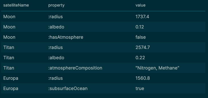
SPARQL

SELECT ?name ?property ?value
WHERE {
  ?s a :NaturalSatellite ;
    :name ?name ;
    ?property ?value .
}

This query would produce results as this (snippet):

SQL: This is impossible without knowing the schema in advance. You’d need to:

• Query the database metadata tables to discover all columns

• Dynamically generate UNION queries for each column

• Handle type conversions (numbers, strings, dates all in one result)

• Write complex application code to reconstruct the results

Another powerful pattern: discovering the schema. What properties do satellites actually have in our dataset?

SPARQL

SELECT DISTINCT ?property
WHERE {
  ?s a :NaturalSatellite ;
    ?property ?value .
}

This gives you an instant inventory of all properties used by satellites in your data. Perfect for data exploration!

Real-world use cases:

• Scientific databases where different experiments measure different properties

• Product catalogs where different product types have different specifications

• Medical records where patients have different test results over time

• IoT data where different sensors report different measurements

• Historical archives where data structure evolved over time

Combining All Three Powers

Here’s where SPARQL really shines, you can combine these features described above for the advanced examples in a single query:

Let’s find all bodies in Jupiter’s orbital system (recursive), enrich with Wikipedia data (federated), and show me whatever properties they have (schema-flexible).

SELECT ?bodyName ?property ?value ?wikiDescription
WHERE {
  # Recursive: anything orbiting Jupiter at any depth
  ?body :orbits+ :Jupiter ;
    :name ?bodyName ;
    ?property ?value .
  
  # Federated: get Wikipedia descriptions
  OPTIONAL {
    SERVICE <http://dbpedia.org/sparql> {
      ?wiki rdfs:label ?bodyName ;
        dbo:abstract ?wikiDescription .
      FILTER(LANG(?wikiDescription) = "en")
    }
  }
}

Try doing that in SQL! This query:

• Recursively traverses orbital relationships

• Queries a remote database on the internet

• Returns flexible properties regardless of schema

• Handles missing Wikipedia entries gracefully with OPTIONAL

💡 Key takeaway: When you combine property paths, federated queries, and schema flexibility, you can answer questions that would require days of programming, ETL work, and database integration in traditional SQL environments.

Try it yourself!

Open SPARQL endpoints:

• DBPedia (includes web-based SPARQL query editor)

• Wikidata (includes web-based SPARQL query editor)

• EU Open Data Portal SPARQL Endpoint

• In Python with maplib

Summary

This article has shown similarities and differences between SQL and SPARQL, and the power that lies within a graph pattern.

From Data Engineering to Knowledge Engineering article-series

Part 1: From Data Engineering to Knowledge Engineering in the blink of an eye
Part 2: Data Engineering Ontologies
Part 3: this
Part 4: From SQL Constraints to SHACL Shapes: Declarative Data Validation